import matplotlib.pyplot as plt
import numpy as np
入门
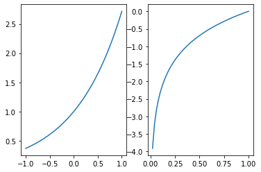
下面,我们将指数函数和对数函数的图像绘制在同一个绘图窗口中。
ex = np.linspace(-1, 1, num=101)
ey = np.exp(ex)

lnx = np.linspace(0.02, 1, num=51)
lny = np.log(lnx)
使用 subplot 可以指定子图的排列方式以及索引。
plt.subplot(121)
plt.plot(ex, ey)

plt.subplot(122)
plt.plot(lnx, lny)
[<matplotlib.lines.Line2D at 0x7fa93eb835d0>]
subplot 返回 Axes 对象。因此,上面的绘图代码也可以这样来写:
ax1 = plt.subplot(121)
ax1.plot(ex, ey)

ax2 = plt.subplot(122)
ax2.plot(lnx, lny)
[<matplotlib.lines.Line2D at 0x7fa93ea6ba50>]

但是,subplot 方法不能够直接返回 Figure 对象,这会在设置 Figure 对象属性的时候造成一些麻烦。因此,我们要介绍更一般的方法。
创建指定排布的子图
在 Matplotlib 中,我们使用 subplots 创建可以指定子图排布的窗口。
fig, ax = plt.subplots()
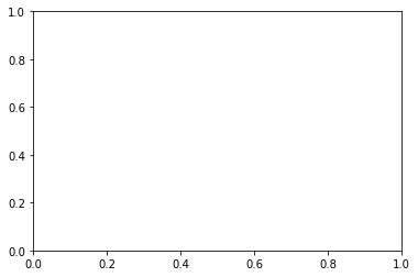
如果不给 subplots 指定任何参数,那么默认就会创建一个 Axes 对象,即只有一个绘图区域。
subplots 函数返回两个值:一是绘图窗口 Figure 对象,二是指向每个子图绘图区域的 Axes 数组。
当然,我们也可以用 Figure 对象来创建子图绘图区域。下面的代码与上面的等价:
fig = plt.figure()
ax = fig.subplots()

一般地,我们在绘制子图时先要确定好子图的排布情况。例如现在我们要绘制 $6$ 幅子图,按照 $2 \times 3$ 排列:
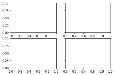
fig, ax = plt.subplots(nrows=2, ncols=3)
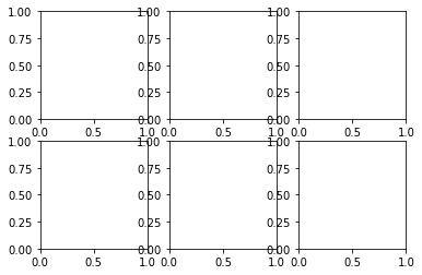
nrows 和 ncols 分别指子图排布的行数和列数。
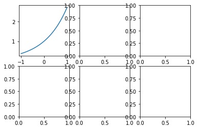
我们通过简单的下标索引就能够确定每个子图绘图区域的 Axes 对象。
ax[0, 0].plot(ex, ey)
fig
如果子图不多,也可以采用下面的方法直接得到每个子图对象,而不需要索引:
fig, (ax1, ax2) = plt.subplots(2, 1)
上面的 Figure 对象只包含 $2$ 个 Axes 子图,可以直接以元祖的形式来接收返回值。
共享坐标轴
sharex 和 sharey 参数分别表示是否共享同一个 $x$ 轴或 $y$ 轴。
fig, (ax1, ax2) = plt.subplots(2, 1, sharex=True)
同理:
fig, (ax1, ax2) = plt.subplots(1, 2, sharey=True)
如果我们的子图排布较为复杂,可以这样来共享坐标轴:
指定每一列共享 $x$ 轴:
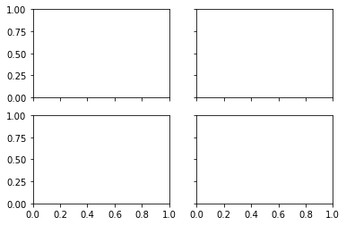
fig, ax = plt.subplots(2, 2, sharex=True)
指定每一行共享 $y$ 轴:
fig, ax = plt.subplots(2, 2, sharey=True)
$x$ 轴和 $y$ 轴均共享:
fig, ax = plt.subplots(2, 2, sharex=True, sharey=True)
自定义布局
如果我们只希望画 $3$ 副子图,又希望其中一副能够完整填充空白区域。一个简单的方法就是直接使用 subplot:
plt.subplot(221)
plt.plot(ex, ey)

plt.subplot(222)
plt.plot(lnx, lny)

plt.subplot(212)
plt.plot(ex, ey)
plt.plot(lnx, lny)
[<matplotlib.lines.Line2D at 0x7fa93e1ec310>]
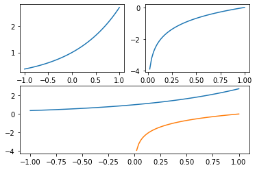
上面代码的前两部分将 Figure 对象看作是 $2 \times 2$ 的矩阵,然后只用到第一行。然后再将 Figure 对象看作是 $2 \times 1$ 的矩阵,然后继续绘制第二行。这种绘制方法较为简单,但是需要确定好布局,否则会出现运行时错误。
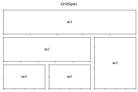
另一种方法是采用 Figure 对象的 add_subplot 方法。首先,我们需要导入 GridSpec 子图布局模块。
from matplotlib.gridspec import GridSpec
首先,我们创建 Figure 对象。最好我们设置它的布局为约束布局,这样当我们在向其中添加一些元素或修改属性时,Matplotlib 会帮助我们自动调整间距,避免重叠。
fig = plt.figure(constrained_layout=True)
<Figure size 432x288 with 0 Axes>
然后,我们创建子图布局对象:
gs = GridSpec(3, 3, figure=fig)
子图布局对象的作用就是辅助我们去构建我们想要的绘图区域 Axes 的形状。配合 Figure 对象的 add_subplot 方法以及矩阵的索引与切片机制,我们可以自由地创建各种各样的 Axes 绘图区域。
ax1 = fig.add_subplot(gs[0, :])
ax2 = fig.add_subplot(gs[1, :-1])
ax3 = fig.add_subplot(gs[1:, -1])
ax4 = fig.add_subplot(gs[-1, 0])
ax5 = fig.add_subplot(gs[-1, -2])

fig
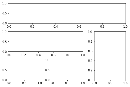
上面的 Figure 的坐标轴数字都没有挤在一起,说明了约束布局的重要性。
我们可以定义下面的函数,稍微美化一下这个绘图窗口:
def format_axes(fig):
    for i, ax in enumerate(fig.axes):
        ax.text(0.5, 0.5, "ax%d" % (i+1), va="center", ha="center")
        ax.tick_params(labelbottom=False, labelleft=False)
结果如下:
format_axes(fig)
fig.suptitle("GridSpec")
fig
子图的属性与窗口的属性
在概述中,我们就强调了 Figure 对象和 Axes 对象的本质不同。而直到学习到绘制子图,我们才能够渐渐地明白子图的属性和窗口的属性是有很大不同的,是会产生不同的效果的。
设置图例
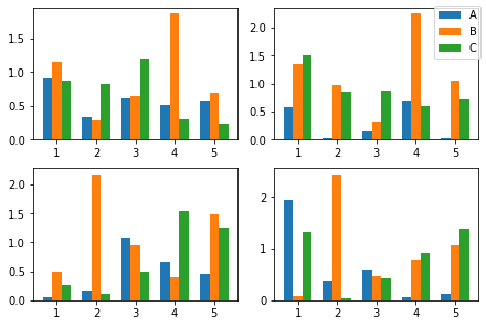
图例的设置是一个非常经典的例子。假设目前我们一共有 $4$ 组数据,每组数据一共有 $3$ 个指标 $5$ 个系列。现在,我们先生成这个 $4 \times 3 \times 5$ 的矩阵。
data = np.abs(np.random.randn(4, 3, 5))
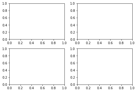
由于一共有 $4$ 组数据,于是我们用 subplots 方法来生成一个 $2 \times 2$ 布局的子图绘制窗口。
fig, ax = plt.subplots(2, 2, constrained_layout=True)
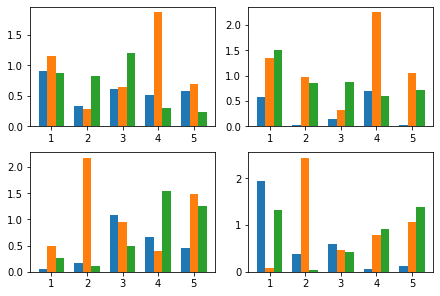
下面绘制系列条形图:
x = np.arange(1, 6)
width = 0.24

ax[0, 0].bar(x - width, data[0, 0, :], width=width, label='A')
ax[0, 0].bar(x, data[0, 1, :], width=width, label='B')
ax[0, 0].bar(x + width, data[0, 2, :], width=width, label='C')

ax[0, 1].bar(x - width, data[1, 0, :], width=width, label='A')
ax[0, 1].bar(x, data[1, 1, :], width=width, label='B')
ax[0, 1].bar(x + width, data[1, 2, :], width=width, label='C')

ax[1, 0].bar(x - width, data[2, 0, :], width=width, label='A')
ax[1, 0].bar(x, data[2, 1, :], width=width, label='B')
ax[1, 0].bar(x + width, data[2, 2, :], width=width, label='C')

ax[1, 1].bar(x - width, data[3, 0, :], width=width, label='A')
ax[1, 1].bar(x, data[3, 1, :], width=width, label='B')
ax[1, 1].bar(x + width, data[3, 2, :], width=width, label='C')

fig
现在,我们给每个子图添加图例:
ax[0, 0].legend()
ax[0, 1].legend()
ax[1, 0].legend()
ax[1, 1].legend()

fig
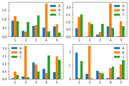
然而,实际上我们没有必要为每个子图都添加图例。这个问题的本质在于,legend 是从属于子图的 Axes 对象,还是从属于 Figure 对象?
如果我们只需要绘制从属于 Figure 对象的一份图例,Figure 对象就必须知道数据和对应的标签,这需要捕获 Bar 对象。
fig, ax = plt.subplots(2, 2, constrained_layout=True)

rects1 = ax[0, 0].bar(x - width, data[0, 0, :], width=width, label='A')
rects2 = ax[0, 0].bar(x, data[0, 1, :], width=width, label='B')
rects3 = ax[0, 0].bar(x + width, data[0, 2, :], width=width, label='C')

ax[0, 1].bar(x - width, data[1, 0, :], width=width, label='A')
ax[0, 1].bar(x, data[1, 1, :], width=width, label='B')
ax[0, 1].bar(x + width, data[1, 2, :], width=width, label='C')

ax[1, 0].bar(x - width, data[2, 0, :], width=width, label='A')
ax[1, 0].bar(x, data[2, 1, :], width=width, label='B')
ax[1, 0].bar(x + width, data[2, 2, :], width=width, label='C')

ax[1, 1].bar(x - width, data[3, 0, :], width=width, label='A')
ax[1, 1].bar(x, data[3, 1, :], width=width, label='B')
ax[1, 1].bar(x + width, data[3, 2, :], width=width, label='C')

lg = fig.legend((rects1, rects2, rects3), ('A', 'B', 'C'))
下面我们来美化一下这个图例。我们希望它显示在窗口右上角,并且不要遮挡图像。
lg.set_bbox_to_anchor(bbox=(0.13, 0, 1, 1))
fig
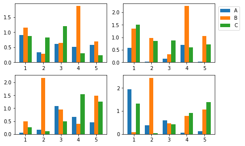
其中,参数 bbox 接收的四元组中,前两个分量分别代表横坐标和纵坐标的相对位置。我们是希望图例向右偏移一些不遮挡图像,因此给横坐标一个较小的增量。后两个分量代表宽和高,一般来说均设置为 $1$,这样不会有任何调整。