Attention Is All You Need
【文献精读】Transformer
Transformer 是目前人工智能和深度学习领域最著名的模型之一,由 Google 团队于 2017 年 6 月提出,发表在 NeuralPS(Conference on Neural Information Processing Systems)上。起初是为了解决自然语言处理(Natural Language Processing, NLP)领域中的机器翻译问题,没想到它的效果竟然超越了循环神经网络(Recurrent Neural Networks, RNN),只需要用 encoder 和 decoder 以及注意力 attention 机制就可以达到很好的效果。
Transformer 本身是专门为 NLP 领域量身定制的,但是后来人们将图像等数据编码和序列化之后同样可以放进 Transformer 中进行训练,并且也能让模型达到和卷积神经网络(Convolutional Neural Networks, CNN)和深度神经网络(Deep Neural Networks, DNN)相比更加出其不意的效果。这才让 Transformer 在计算机视觉领域大火了起来。
特别鸣谢
本文结合亚马逊首席科学家李沐的深度学习论文精读系列视频进行整理。
这篇文章最具特色的就是标题 Attention Is All You Need,翻译成中文就是“你需要注意”。后来这个标题成为了一个梗,即 xxx Is All You Need。
值得注意的是,这篇文章的每一位作者后面都打了 * 号,这说明这几位作者的贡献是均等的,论文首先下的注释已经充分说明了这一点。通常我们会认为论文的第一作者是主要贡献者,但是这篇文章是个例外。
Table of Contents
Abstract
The dominant sequence transduction models are based on complex recurrent or convolutional neural networks that include an encoder and a decoder. The best performing models also connect the encoder and decoder through an attention mechanism. We propose a new simple network architecture, the Transformer, based solely on attention mechanisms, dispensing with recurrence and convolutions entirely. Experiments on two machine translation tasks show these models to be superior in quality while being more parallelizable and requiring significantly less time to train. Our model achieves 28.4 BLEU on the WMT 2014 Englishto-German translation task, improving over the existing best results, including ensembles, by over 2 BLEU. On the WMT 2014 English-to-French translation task, our model establishes a new single-model state-of-the-art BLEU score of 41.0 after training for 3.5 days on eight GPUs, a small fraction of the training costs of the best models from the literature.
所谓序列转录模型 sequence transduction models 是指输入为一个序列,输出也为一个序列的模型。例如在机器翻译中,输入一段中文,然后输出其对应的英文翻译。当时(作者写这篇文章的时候),主流的序列转录模型主要基于复杂的 CNN 和 RNN,一般采用 encoder 和 decoder 架构。作者提出了一种基于注意力机制 attention mechanisms 的网络结构 Transformer。作者做了两个机器翻译的实验,证明了他们提出的模型效果非常好。
7 Conclusion
In this work, we presented the Transformer, the first sequence transduction model based entirely on attention, replacing the recurrent layers most commonly used in encoder-decoder architectures with multi-headed self-attention.
For translation tasks, the Transformer can be trained significantly faster than architectures based on recurrent or convolutional layers. On both WMT 2014 English-to-German and WMT 2014 English-to-French translation tasks, we achieve a new state of the art. In the former task our best model outperforms even all previously reported ensembles.
We are excited about the future of attention-based models and plan to apply them to other tasks. We plan to extend the Transformer to problems involving input and output modalities other than text and to investigate local, restricted attention mechanisms to efficiently handle large inputs and outputs such as images, audio and video. Making generation less sequential is another research goals of ours.
按照沐神读论文的习惯,摘要读完以后直接跳到结论。沐神总结的结论主要有如下几点:
- Transformer 是当时第一个完全基于注意力的序列转录模型,它把过去常用的循环层全部换成了
multi-headed self-attention。 - Transformer 在机器翻译的任务中比基于循环层和卷积层的架构要快很多。
- Transformer 未来可以用在文本以外的数据类型上,例如图像、音频、视频等。现在看来,作者在当时多多少少是预测到未来的研究方向的,我十分佩服!
1 Introduction
这篇文章的导言 Introduction 相对来说比较短,基本上是摘要 Abstract 的扩充。
Recurrent neural networks, long short-term memory1 and gated recurrent2 neural networks in particular, have been firmly established as state of the art approaches in sequence modeling and transduction problems such as language modeling and machine translation. Numerous efforts have since continued to push the boundaries of recurrent language models and encoder-decoder architectures.
当时机器翻译最常用的模型是 RNN,主要包括如下两个著名的网络模型:
- LSTM (Long Short-Term Memory): 长短期记忆网络。它是一种时间循环神经网络,是为了解决一般的 RNN 存在的长期依赖问题而专门设计出来的,所有的 RNN 都具有一种重复神经网络模块的链式形式。
- GRU (Gate Recurrent Unit): 门控循环单元。是 LSTM 网络的一种效果很好的变体,它较 LSTM 网络的结构更加简单,而且效果也很好,因此也是当前非常流形的一种网络。
后续的工作主要围绕着循环语言模型 recurrent language models 和编码器/解码器 encoder-decoder 架构展开。
Recurrent models typically factor computation along the symbol positions of the input and output sequences.
RNN 的特点是序列从左向右移一步一步往前做。当前时刻 $t$ 的隐藏状态 hidden states 记作 $h_t$,它由上一个隐藏状态 $h_{t-1}$ 和当前时刻 $t$ 的输入决定。这就是为什么 RNN 能够处理时序信息的原因。也正因为 RNN 的这一特点,导致 RNN 存在如下问题:
- 计算难以并行,主流的多线程 GPU 只能按照时序一个一个计算。
- 序列长度和 $h_t$ 的长度之间的矛盾。如果序列长度特别长而 $h_t$ 不够长的话,前面的信息很可能会丢掉;但如果 $h_t$ 也设计得很长的话,内存开销太大。
针对 RNN 的这些问题,近年来的改进工作很多,但都没有从根本上解决问题。
Attention mechanisms have become an integral part of compelling sequence modeling and transduction models in various tasks, allowing modeling of dependencies without regard to their distance in the input or output sequences.
注意力机制并不是本文的创新点。在现有的工作中,注意力机制已经被成功地用在编码器/解码器里面了。
In this work we propose the Transformer, a model architecture eschewing recurrence and instead relying entirely on an attention mechanism to draw global dependencies between input and output. The Transformer allows for significantly more parallelization and can reach a new state of the art in translation quality after being trained for as little as twelve hours on eight P100 GPUs.
作者在本文提出的 Transformer 则与 RNN 不同,是完全依赖注意力机制的一种模型架构。作者特别强调了他们在训练时候的并行性 parallelization。
2 Background
The goal of reducing sequential computation also forms the foundation of the Extended Neural GPU, ByteNet and ConvS2S, all of which use convolutional neural networks as basic building block, computing hidden representations in parallel for all input and output positions.
In the Transformer this is reduced to a constant number of operations, albeit at the cost of reduced effective resolution due to averaging attention-weighted positions, an effect we counteract with Multi-Head Attention as described in section 3.2.
为了解决 RNN 训练的并行性问题,有很多工作考虑采用 CNN 来代替 RNN 以增加并行性,但问题是 CNN 对长序列难以建模。例如相隔很远的两个像素块,需要多层卷积才能建立起联系。不过卷积计算的好处是可以做多个输出通道,基于此作者提出了多头注意力 Multi-Head Attention 机制。
Self-attention, sometimes called intra-attention is an attention mechanism relating different positions of a single sequence in order to compute a representation of the sequence.
接下来就是自注意力 Self-attention 机制,这其实也是 Transformer 中很重要的一点。不过该工作并不是 Transformer 的创新点,已经有不少相关工作了。
3 Model Architecture
为了解释清楚 encoder-decoder,作者首先给出如下 3 个非常重要的定义:
- $\left(x_1, x_2, …, x_n\right)$:表示一个序列。假设这个序列是一个英文句子,那么 $x_t$ 就表示第 $t$ 个单词。
- $\textbf{z} = \left(z_1, z_2, …, z_n\right)$:编码器的输出。$z_t$ 是 $x_t$ 的一个向量表示。
- $\left(y_1, y_2, …, y_m\right)$:编码器的输出,是一个长为 $m$ 的序列。和编码器不同的是,解码器的词是一个个生成的,这叫做自回归
auto-regressive。自回归的意思是当前的输出也会作为输入参与下一轮的输出。换句话说就是,翻译的结果出来是一个个词往外蹦儿的。
这样也就弄清楚 Transformer 的输入和输出了,后文则主要对这里面的每个块进行说明。
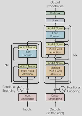
3.1 Encoder and Decoder Stacks
Encoder
- layers: $N=6$
- sub-layers:
- multi-head self-attention mechanism: 多头自注意力机制
- position-wise fully connected feed-forward network: 本质上就是一个 MLP(多层感知机,Multilayer Perceptron)
- output: $\textrm{LayerNorm}(x + \textrm{Sublayer}(x))$
- dimension: $d_{model} = 512$
BatchNorm 和 LayerNorm 的区别
沐神就 BatchNorm 和 LayerNorm 的区别作了详细讲解。我们知道,Norm 即 Normalization,对数据进行归一化处理。这和概率论中对随机变量进行标准化的操作类似,即把原向量化为均值为 $0$ 方差为 $1$ 的标准化向量。
$$ \begin{align*} Y = \frac{X - \mu}{\sigma} \end{align*} $$
如图所示,BatchNorm 和 LayerNorm 的区别一目了然。BatchNorm 是在每一个特征 feature 上对 batch 进行归一化,而 LayerNorm 是在每一个样本 batch 上对 feature 进行归一化。
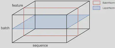
为什么要使用 LayerNorm 呢?一个原因是样本长度可能发生变化(即 sequence 的长度 $n$),如果使用 BatchNorm 的话,切片的结果可能长度参差不齐,会有很多零填充。而使用 LayerNorm 则不会出现这样的问题,因为是同一个样本(即同一个序列)。由于序列长度不一有零填充,计算均值和方差的时候每个样本的计算方法不一样,不能把零算进去,因为零不是有效值。
还有一点原因是,假如在做预测的时候,序列特别特别长以至于训练所得的均值和方差并不好用。而使用 LayerNorm 则不会出现这样的问题,因为它是每个样本独立计算的,最后也并不像 BatchNorm 那样需要算出一个全局的均值和方差。因此不管序列有多长,均值和方差都是在序列本身的基础上算的。
Decoder
- layers: $N=6$
- sub-layers:
- multi-head self-attention mechanism: 和
encoder相同 - position-wise fully connected feed-forward network: 和
encoder相同 - masked multi-head attention: 带掩码的多头注意力机制
- multi-head self-attention mechanism: 和
- masking: 确保位置 $i$ 的预测只能依赖于小于 $i$ 位置的已知输出。因为训练时
decoder的输入是上面一些时刻在encoder的输出,不应该看到后面时刻的输入。
3.2 Attention
An attention function can be described as mapping a query and a set of key-value pairs to an output, where the query, keys, values, and output are all vectors. The output is computed as a weighted sum of the values, where the weight assigned to each value is computed by a compatibility function of the query with the corresponding key.
注意力函数是将 query 和一些键值对 key-value pairs 映射成一个输出 output 的函数,这里面的 query、keys、values、output 都是向量 vectors。具体来说,output 是 values 的加权,其输出维度和 value 的维度是一样的。权重是通过每个 value 对应的 key 和 query 计算相似度 compatibility function 得来的。这里的相似度针对不同的注意力机制有不同的算法。
3.2.1 Scaled Dot-Product Attention
作者在本小节主要说明了 Transformer 采用的注意力机制。作者将之命名为 Scaled Dot-Product Attention,如图所示。
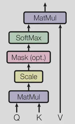
注意力函数的计算公式如下:
$$ \begin{align*} \textrm{Attention}\left(Q, K, V\right) = \textrm{softmax}\left(\frac{QK^{\top}}{\sqrt{d_k}}\right)V \end{align*} $$$Q$ 即 query,$K$ 即 key,$QK^{\top}$ 即 query 和 key 做内积。作者认为,两个向量的内积值越大,说明相似度越高。除以 $\sqrt{d_k}$ 则表示单位化,然后再用 softmax 得到权重。这里的道理其实就是机器学习中的余弦相似度(余弦距离):
注意这里 Mask 的作用是为了避免 $t$ 时刻看到后面的输入。在数学上的具体实现方式是以一个绝对值非常大的负数($-\infty$)作为指数,计算出来的幂趋向于零,这样就实现了掩盖 $t$ 时刻后面的输入的效果。
3.2.2 Multi-Head Attention
作者认为,与其计算单个的注意力函数,不如把 query、key、value 投影到一个更低的维度上,投影 $h$ 次,然后再计算 $h$ 次注意力函数,最后每一个函数的输出合并再投影得到最终的输出。如图所示。
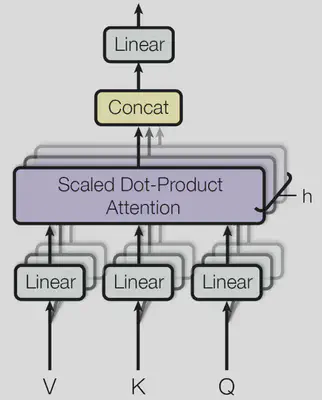
多头注意力函数的计算公式如下:
$$ \begin{align*} \textrm{MultiHead}\left(Q, K, V\right) &= \textrm{Concat}\left(\textrm{head}_1, ..., \textrm{head}_h\right)W^O \\\\ \textbf{where}\quad\textrm{head}_i &= \textrm{Attention}\left(QW^Q_i, KW^K_i, VW^V_i\right) \end{align*} $$在本文中作者定义 $h=8$,于是 $d_k = d_v = d_{model}/h = 64$,也就是输出维度。
3.2.3 Applications of Attention in our Model
这一小节作者主要介绍 Transformer 是如何使用注意力的,归结起来一共有如下 3 种情况:
In “encoder-decoder attention” layers, the queries come from the previous decoder layer, and the memory keys and values come from the output of the encoder. This allows every position in the decoder to attend over all positions in the input sequence.
The encoder contains self-attention layers. In a self-attention layer all of the keys, values and queries come from the same place, in this case, the output of the previous layer in the encoder. Each position in the encoder can attend to all positions in the previous layer of the encoder.
Similarly, self-attention layers in the decoder allow each position in the decoder to attend to all positions in the decoder up to and including that position. We need to prevent leftward information flow in the decoder to preserve the auto-regressive property. We implement this inside of scaled dot-product attention by masking out (setting to $-\infty$) all values in the input of the softmax which correspond to illegal connections.
encoder的Multi-Head Attention以key、value、query作为输入。图中的箭头一分为三,表示同一数据复制三次,这就叫做自注意力机制。输出的维度和输入一致。decoder的Masked Multi-Head Attention和encoder的Multi-Head Attention类似,只不过需要掩盖后面的输入,前文已详述。decoder的Multi-Head Attention则不再像encoder那样是自注意力了,而是key和value来自于编码器的输出,query来自于解码器下一个attention的输入。
为了更便于大家理解,沐神举了一个非常简单的机器翻译的例子:
Hello world
你好世界
显然,输入的英文序列 $n=2$,输出的中文序列 $m=4$。当 Transformer 在计算“好”字时,把“好”字对应的向量作为 query 时,计算和 Hello 对应的向量的相似度会更高一些,就会赋一个较大的权重。这就是注意力机制给我们最直观的感受!
3.3 Position-wise Feed-Forward Networks
$$ \begin{align*} \textrm{FFN}\left(x\right) = \max \left(0, xW_1 + b_1\right)W_2 + b_2 \end{align*} $$In addition to attention sub-layers, each of the layers in our encoder and decoder contains a fully connected feed-forward network, which is applied to each position separately and identically. This consists of two linear transformations with a ReLU activation in between.
在注意力层之后,encoder 和 decoder 都会有一个前馈网络层,首先是一个全连接层,然后是 ReLU 激活函数,最后再过一个全连接层。
3.4 Embeddings and Softmax
Similarly to other sequence transduction models, we use learned embeddings to convert the input tokens and output tokens to vectors of dimension $d_{model}$. We also use the usual learned linear transformation and softmax function to convert the decoder output to predicted next-token probabilities.
Embeddings 将输入的每一个词 token 映射成维度为 $d_{model}$ 的向量。Softmax 的作用是归一化。
3.5 Positional Encoding
Since our model contains no recurrence and no convolution, in order for the model to make use of the order of the sequence, we must inject some information about the relative or absolute position of the tokens in the sequence. To this end, we add “positional encodings” to the input embeddings at the bottoms of the encoder and decoder stacks. The positional encodings have the same dimension $d_{model}$ as the embeddings, so that the two can be summed.
为什么需要位置编码呢?因为 attention 本身并没有时序信息,它只是计算了 key 和 query 之间的余弦距离,它与序列的时序性无关。例如我们阅读下面这句话:
序语倒颠不响影读阅。
我们会觉得有些别扭,因为语义发生变化了。但其实 attention 在计算的时候根本处理不了这种情况,这个时候就需要把时序信息加进来。与 RNN 不同的是,Transformer 在输入里面加入时序信息,而 RNN 则是以上一时刻的输出作为部分输入。
4 Why Self-Attention
本节作者介绍了为什么要采用自注意力机制。沐神认为,作者并没有把这个原因讲得特别清楚。不过,我们可以首先来看看下表:
| Layer Type | Complexity per Layer | Sequential Operations | Maximum Path Length |
|---|---|---|---|
| Self-Attention | $O(n^2 \cdot d)$ | $O(1)$ | $O(1)$ |
| Recurrent | $O(n \cdot d^2)$ | $O(n)$ | $O(n)$ |
| Convolutional | $O(k \cdot n \cdot d^2)$ | $O(1)$ | $O(\log_k{n})$ |
| Self-Attention (restricted) | $O(r \cdot n \cdot d)$ | $O(1)$ | $O(n/r)$ |
作者对比了自注意力机制、RNN、CNN 和受限制的 restricted 自注意力机制的三个方面:计算复杂度、顺序计算、最大路径长度。显然计算复杂度越低越好;顺序计算是指下一步计算必须等前面几步计算完成才能计算,当然越低越好,并行度越高;最大路径长度是指一个序列信息从一个数据点走到另一个数据点需要走多远,当然越短越好。
这里需要额外解释的是受限制的自注意力机制。为什么相比与自注意力机制,其计算复杂度会有所降低?是因为 query 只跟最近的 $r$ 个邻居做运算。但带来的问题是最大路径长度的增加。
5 Training
5.1 Training Data and Batching
5.2 Hardware and Schedule
5.3 Optimizer
5.4 Regularization
6 Results
6.1 Machine Translation
6.2 Model Variations
Bowen Zhou
Student pursuing a PhD degree of Computer Science and Technology
My research interests include Edge Computing and Edge Intelligence.