
仿射集合和凸集
直线与线段
设
组成一条穿越
构成了
还有如下一种表示形式,它类似于直线的参数方程:
仿射集合
如果通过集合
这个概念可以推广至多个点的情况:如果
设
与仿射集合
我们称由集合
仿射包是包含
仿射维数与相对内部
集合
考虑
其仿射包为
凸集
若对
则称集合
INFO
仿射集合是凸集
由于仿射集包含穿过集合中任意不同两点的整条直线,任意不同两点间的线段自然也在集合中,因而仿射集是凸集。
TikZ 代码
\begin{tikzpicture}[line cap=round,line join=round,scale=0.9]
  % convex hexagon
  \draw[fill=gray!20]
    (0.95,0) -- (0.47,0.82) -- (-0.47,0.82) -- (-0.95,0) -- (-0.47,-0.82) -- (0.47,-0.82) -- cycle;
  % nonconvex kidney-like set with a chord escaping the set
  \begin{scope}[shift={(3.4,0)},scale=1.05]
    \draw[fill=gray!20] plot[smooth cycle,tension=1]
      coordinates {(0,1.05) (1.35,0.95) (1.55,-0.15) (1.05,-1.0) (0.62,-0.28)
                   (0.18,-0.1) (-0.15,-0.95) (-1.1,-0.5) (-1.15,0.6)};
    \fill (0.15,0.1) circle (1.3pt);
    \fill (1.45,0.55) circle (1.3pt);
    \draw (0.15,0.1) -- (1.45,0.55);
  \end{scope}
  % square with parts of its boundary missing (not convex)
  \begin{scope}[shift={(6.6,0)}]
    \draw[fill=gray!20] (-0.95,-0.95) rectangle (0.95,0.95);
    \draw[line width=3pt,white] (-0.95,0.55) -- (-0.95,0.1);
    \draw[line width=3pt,white] (0.35,0.95) -- (0.8,0.95);
    \draw[line width=3pt,white] (0.95,-0.15) -- (0.95,0.3);
    \draw[line width=3pt,white] (-0.5,-0.95) -- (-0.05,-0.95);
  \end{scope}
\end{tikzpicture}
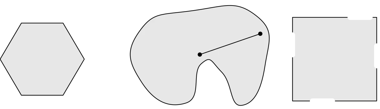
如图所示,左边的正六边形是凸集;中间的图形不是凸集,因为任意两点之间的连线不一定都被集合包含;右边的正方形也不是凸集,因为它仅包含部分边界。
我们称
我们称集合
TikZ 代码
\begin{tikzpicture}[line cap=round,line join=round,scale=0.9]
  % left: convex hull of finitely many points
  \begin{scope}
    \draw[fill=gray!20] (0.15,0.1) -- (0.6,1.35) -- (2.3,1.5) -- (2.45,0.6) -- (1.55,-0.05) -- cycle;
    \foreach \p in {(0.15,0.1),(0.6,1.35),(2.3,1.5),(2.45,0.6),(1.55,-0.05)}
      \fill \p circle (1.4pt);
    \foreach \p in {(0.75,0.75),(1.15,0.5),(1.5,0.95),(1.9,1.1),(0.9,1.1),(1.3,0.15),(1.75,0.45),(2.0,0.75)}
      \fill \p circle (1.2pt);
  \end{scope}
  % right: convex hull of a nonconvex set fills in its concavities
  \begin{scope}[shift={(5.2,0)},scale=1.05]
    \draw[fill=gray!20] plot[smooth cycle,tension=0.75]
      coordinates {(0.0,0.65) (0.7,1.4) (1.65,1.4) (2.2,0.9) (2.05,0.35)
                   (1.2,0.05) (0.35,0.1)};
    \draw plot[smooth cycle,tension=0.5]
      coordinates {(0.25,0.62) (0.75,1.22) (1.6,1.28) (2.02,0.85) (1.75,0.55)
                   (1.3,0.75) (1.05,0.35) (0.78,0.27) (0.45,0.32)};
  \end{scope}
\end{tikzpicture}
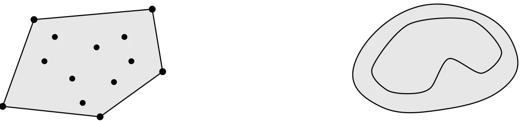
如图所示,左边的一系列散点的凸包是外层散点连线所构成的多边形;右边的图形的凸包是用与图形相切的部分代替凹陷的部分重新构成的封闭图形。凸包是包含
凸组合的概念可以扩展到无穷级数、积分以及大多数形式的概率分布。例如:
锥
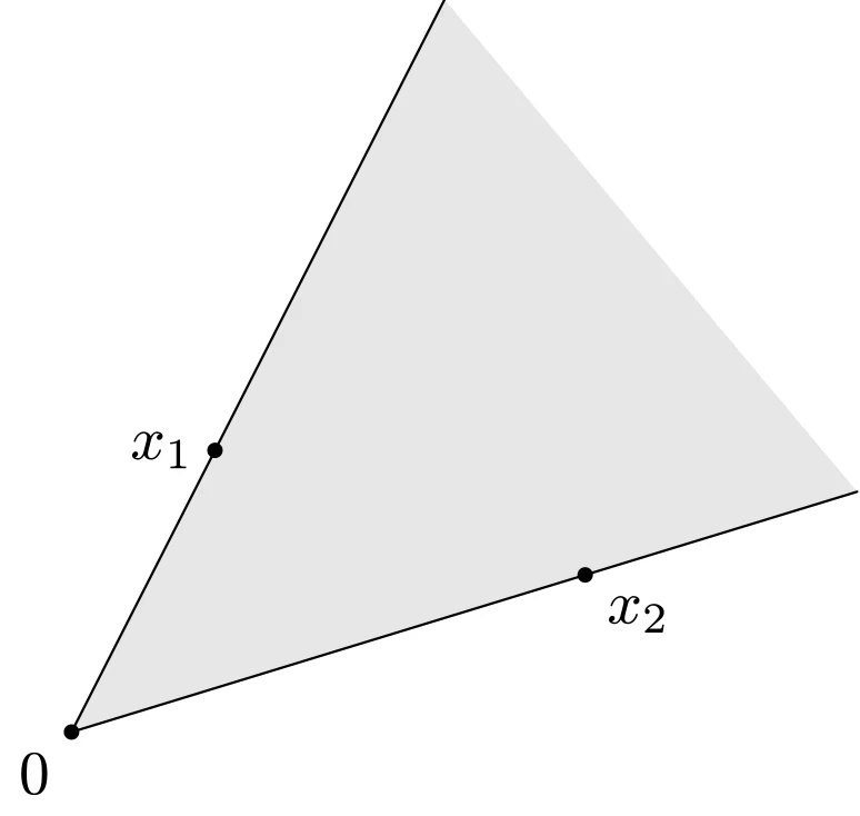
如果对
半径为
TikZ 代码
\begin{tikzpicture}[line cap=round,line join=round,scale=0.9]
  \coordinate (O) at (0,0);
  \coordinate (A) at (63:5.2);
  \coordinate (B) at (17:5.2);
  \fill[gray!20] (O) -- (A) -- (B) -- cycle;
  \draw (O) -- (A);
  \draw (O) -- (B);
  \fill (O) circle (1.4pt) node[below left] {$0$};
  \fill (63:2.0) circle (1.4pt) node[left] {$x_1$};
  \fill (17:3.4) circle (1.4pt) node[below right] {$x_2$};
\end{tikzpicture}
例如,半空间
和凸组合和凸包类似,可以定义锥组合和锥包。集合
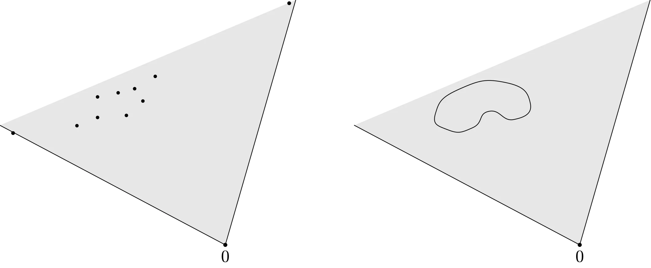
锥包是包含
TikZ 代码
\begin{tikzpicture}[line cap=round,line join=round,scale=0.85]
  % left: conic hull of finitely many points
  \begin{scope}
    \coordinate (O) at (4.6,-2.6);
    \coordinate (A) at (-0.87,0.31);
    \coordinate (B) at (6.31,3.36);
    \fill[gray!20] (O) -- (A) -- (B) -- cycle;
    \draw (O) -- (A);
    \draw (O) -- (B);
    \fill (O) circle (1.4pt) node[below] {$0$};
    \fill (-0.55,0.12) circle (1.3pt);
    \fill (6.15,3.28) circle (1.3pt);
    \foreach \p in {(1.5,1.0),(2.0,1.1),(2.6,0.9),(1.5,0.5),(2.2,0.55),(2.9,1.5),(1.0,0.3),(2.4,1.2)}
      \fill \p circle (1.2pt);
  \end{scope}
  % right: conic hull of a nonconvex set
  \begin{scope}[shift={(8.6,0)}]
    \coordinate (O) at (4.6,-2.6);
    \coordinate (A) at (-0.87,0.31);
    \coordinate (B) at (6.31,3.36);
    \fill[gray!20] (O) -- (A) -- (B) -- cycle;
    \draw (O) -- (A);
    \draw (O) -- (B);
    \fill (O) circle (1.4pt) node[below] {$0$};
    \draw plot[smooth cycle,tension=1]
      coordinates {(1.0,0.9) (1.7,1.75) (2.8,1.8) (3.4,1.2) (3.0,0.75)
                   (2.4,0.95) (2.0,0.5) (1.4,0.45)};
  \end{scope}
\end{tikzpicture}
小结
| 仿射集 | 凸集 | 锥 | 凸锥 |
|---|---|---|---|
| 仿射组合 | 凸组合 | 锥组合 |
|---|---|---|
| 仿射包 | 凸包 | 锥包 |
|---|---|---|