Lagrange 对偶函数

Lagrange 函数

考虑标准形式的优化问题

$$\begin{array}{rl}\mathrm{minimize}& f_0(x)\\ \mathrm{subject}\mathrm{to}& f_i(x)⩽0,i=1,\cdots ,m\\ & h_i(x)=0,i=1,\cdots ,p\end{array}$$

定义该问题的 Lagrange 函数 $L:{\mathbf{R}}^n\times {\mathbf{R}}^m{\mathbf{R}}^p\to \mathbf{R}$ 为

$$L(x,\lambda ,\nu )=f_0(x)+\sum _{i=1}^m{\lambda }_i{f}_i(x)+\sum _{i=1}^p{\nu }_i{h}_i(x)$$

其中定义域 $\mathrm{dom}L=\mathcal{D}\times {\mathbf{R}}^m\times {\mathbf{R}}^p$。${\lambda }_i$ 称为第 $i$ 个不等式约束 $f_i(x)⩽0$ 对应的 Lagrange 乘子；类似地，${\nu }_i$ 称为第 $i$ 个等式约束 $h_i(x)=0$ 对应的 Lagrange 乘子。向量 $\lambda$ 和 $\nu$ 称为对偶变量或者问题的 Lagrange 乘子向量。

Lagrange 对偶函数

定义 Lagrange 对偶函数 $g:{\mathbf{R}}^m\times {\mathbf{R}}^p\to \mathbf{R}$ 为 Lagrange 函数关于 $x$ 取得的最小值：即对 $\lambda \in {\mathbf{R}}^m$，$\nu \in {\mathbf{R}}^p$，有

$$g(\lambda ,\nu )=\underset{x\in \mathcal{D}}{inf}L(x,\lambda ,\nu )=\underset{x\in \mathcal{D}}{inf}(f_0(x)+\sum _{i=1}^m{\lambda }_i{f}_i(x)+\sum _{i=1}^p{\nu }_i{h}_i(x))$$

如果 Lagrange 函数关于 $x$ 无下界，则对偶函数取值为 $-\mathrm{\infty }$。因为对偶函数是一族关于 $(\lambda ,\nu )$ 的仿射函数的逐点下确界，所以即使原问题不是凸的，对偶函数也是凹函数。

最优值的下界

对偶函数构成了原问题最优值 $p^{\star }$ 的下界：即对 $\mathrm{\forall }\lambda ,\nu ⪰0$ 有

$$g(\lambda ,\nu )⩽p^{\star }$$

几何意义

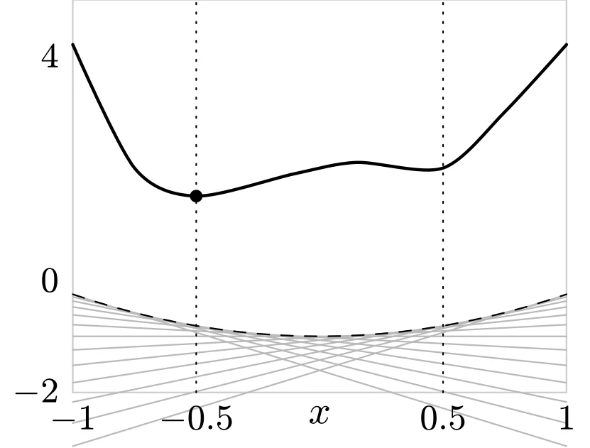
为了便于理解，我们考虑只有一个变量 $x\in \mathbf{R}$ 并且只有一个不等式约束的简单情形。如下图所示：

TikZ 代码

\begin{tikzpicture}[x=2.2cm,y=0.5cm,line cap=round]
  % family of lines f0 + lambda f1, the solid f0 and the dashed lower envelope
  \draw[gray!40] (-1,-2) rectangle (1,5);
  \foreach \t in {-0.9,-0.75,...,0.9}
    \draw[gray!55] plot[domain=-1:1] (\x, {1.5*\t*\x - 0.75*\t*\t - 1});
  \draw[dashed] plot[domain=-1:1] (\x, {0.75*\x*\x - 1});
  \draw[thick] plot[smooth] coordinates {(-1,4.2) (-0.75,2.0) (-0.5,1.5) (-0.1,1.9) (0.15,2.1) (0.5,2.0) (0.75,3.0) (1,4.2)};
  \draw[dotted] (-0.5,-2) -- (-0.5,5);
  \draw[dotted] (0.5,-2) -- (0.5,5);
  \fill (-0.5,1.5) circle (1.6pt);
  \node[below] at (0,-2) {$x$};
  \node[left] at (-1,4) {\small $4$};
  \node[left] at (-1,0) {\small $0$};
  \node[left] at (-1,-2) {\small $-2$};
  \node[below] at (-1,-2) {\small $-1$};
  \node[below] at (-0.5,-2) {\small $-0.5$};
  \node[below] at (0.5,-2) {\small $0.5$};
  \node[below] at (1,-2) {\small $1$};
\end{tikzpicture}

图中表示的是对偶可行点给出的下界。粗的实线表示目标函数 $f_0$，下方的虚线表示约束函数 $f_1$。可行集是图中两个红点之间的部分所在区间。细的点线表示一系列 Lagrange 函数 $L(x,\lambda )$，其中 $\lambda ={\lambda }_1,{\lambda }_2,{\lambda }_3,\cdots$。该问题的最优点是左边的红点所在位置，可以看到每个 Lagrange 函数的极小值均小于之。

通过线性逼近来理解

可以通过对集合 $\{0\}$ 和 $-{\mathbf{R}}_{+}$ 的示性函数进行线性逼近来理解 Lagrange 函数和其给出下界的性质。首先将原问题重新描述成一个无约束问题

$$\mathrm{minimize}{f}_0(x)+\sum _{i=1}^m{I}_{-}(f_i(x))+\sum _{i=1}^p{I}_0(h_i(x))$$

其中，$I_{-}:\mathbf{R}\to \mathbf{R}$ 是非正实数集的示性函数

$$I_{-}(u)=\{\begin{array}{cc}0& u⩽0\\ \mathrm{\infty }& u>0\end{array}$$

类似地，$I_0$ 是集合 $\{0\}$ 的示性函数。打一个形象的比喻，可以将函数 $I_{-}(u)$ 理解为我们对约束函数值 $u=f_i(x)$ 的一种恼怒或不满。类似地，$I_0(u)$ 表达了我们对等式约束值 $u=h_i(x)$ 的不满。

如果我们用线性函数 ${\lambda }_i(u)$ 替代函数 $I_{-}(u)$，其中 ${\lambda }_i⩾0$，用函数 ${\nu }_{i}u$ 替代 $I_0(u)$。那么，目标函数就变成了 Lagrange 函数 $L(x,\lambda ,\nu )$，且对偶函数值是该问题的最优值。实际上，使用线性函数太“软”，没有示性函数“硬”。用线性函数去逼近示性函数是远远不够的，不过至少可以将线性函数看作是示性函数的一个下估计。

用“软”约束代替“硬”约束的思想在后文考虑内点法时会再次提到。

举例

线性方程组的最小二乘解

$$\begin{array}{rl}\mathrm{minimize}& x^{\mathrm{\top }}x\\ \mathrm{subject}\mathrm{to}& Ax=b\end{array}$$

其中 $A\in {\mathbf{R}}^{p\times n}$，说明这个问题共有 $p$ 个等式约束。其 Lagrange 函数和对偶函数分别为

$$\begin{array}{rl}L(x,\nu )& =x^{\mathrm{\top }}x+{\nu }^{\mathrm{\top }}(Ax-b)\\ g(\nu )& =\underset{x}{inf}L(x,\nu )\end{array}$$

由于 $L(x,\nu )$ 是关于 $x$ 的二次凸函数，可以通过求解如下最优性条件得到函数的最小值

$$\begin{array}{rl}{\mathrm{\nabla }}_{x}L(x,\nu )=2x+A^{\mathrm{\top }}\nu & =0\\ x& =-{\displaystyle \frac{1}{2}}{A}^{\mathrm{\top }}\nu \end{array}$$

因此，对偶函数为

$$g(\nu )=-{\displaystyle \frac{1}{4}}{\nu }^{\mathrm{\top }}A{A}^{\mathrm{\top }}\nu -b^{\mathrm{\top }}\nu$$

它是一个二次凹函数，定义域为 ${\mathbf{R}}^p$。

Lagrange 对偶函数和共轭函数

共轭函数和 Lagrange 对偶函数紧密相关。下面的问题说明了一个简单的联系。

$$\begin{array}{rl}\mathrm{minimize}& f(x)\\ \mathrm{subject}\mathrm{to}& x=0\end{array}$$

虽然这个问题没有什么挑战性，但是我们还是可以很容易地得到 Lagrange 函数为 $L(x,\nu )=f(x)+{\nu }^{\mathrm{\top }}x$，则其对偶函数为

$$g(\nu )=\underset{x}{inf}(f(x)+{\nu }^{\mathrm{\top }}x)=-\underset{x}{sup}((-\nu {)}^{\mathrm{\top }}x-f(x))=-f^{\ast }(-\nu )$$

即，我们得到了结论

$$g(\nu )=-f^{\ast }(-\nu )$$