自和谐

经典的 Newton 方法收敛分析（基于强凸性与 Hessian 的 Lipschitz 连续性）有两个主要缺点。第一个是实际层面的：所得的复杂度估计涉及三个常数 $m$、$M$ 和 $L$，而这些常数在实践中几乎总是未知的，因此迭代次数的上界几乎无法具体给出。当然，收敛分析本身在概念上仍然有用。第二个缺点是：尽管 Newton 方法本身是仿射不变的，经典分析却强烈依赖于坐标系——改变坐标会使 $m$、$M$ 和 $L$ 全部改变。因此，我们希望找到一种像 Newton 方法本身一样独立于仿射坐标变换的分析。

Nesterov 和 Nemirovski 发现了一个能够实现这一目标的简单而优雅的假设，并称之为自和谐​（self-concordance）。自和谐函数之所以重要，有以下几个原因：

• 其中包括许多在凸优化内点法中起重要作用的对数障碍函数。
• 对自和谐函数的 Newton 方法分析不依赖任何未知常数。
• 自和谐是仿射不变的性质：对自和谐函数做线性变换后得到的仍是自和谐函数，因此对 Newton 方法给出的复杂度估计独立于仿射坐标变换。

定义与例子

$\mathbf{R}$ 上的自和谐函数

先考虑 $\mathbf{R}$ 上的函数。凸函数 $f:\mathbf{R}\to \mathbf{R}$ 称为自和谐的，如果

$$|f^{‴}(x)|⩽2f^{″}(x{)}^{3/2}$$

对所有 $x\in \mathrm{dom}f$ 成立。线性函数与（凸）二次函数的三阶导数为零，显然是自和谐的。更多例子：

• 负对数​：$f(x)=-\log x$ 是自和谐的。由 $f^{″}(x)=1/x^2$，$f^{‴}(x)=-2/x^3$，可得 $|f^{‴}(x)|/(2f^{″}(x{)}^{3/2})=1$，定义不等式以等号成立。
• 负熵加负对数​：$f(x)=x\log x-\log x$ 是自和谐的。由 $f^{″}(x)=(x+1)/x^2$，$f^{‴}(x)=-(x+2)/x^3$，可得 $|f^{‴}(x)|/(2f^{″}(x{)}^{3/2})=(x+2)/(2(x+1{)}^{3/2})$，该函数在 ${\mathbf{R}}_{+}$ 上的最大值为 1（在 $x=0$ 处取得）。单独的负熵函数不是自和谐的。

关于定义中的常数 2，需要作一点说明：这个常数只是为方便而选的，目的是简化后面的公式；任何其他正常数都可以。若凸函数满足 $|f^{‴}(x)|⩽k{f}^{″}(x{)}^{3/2}$（$k$ 为某正常数），则 $\tilde{f}(x)=(k^2/4)f(x)$ 满足标准自和谐不等式。因此重要的是：函数的三阶导数被其二阶导数的 3/2 次幂的某个倍数控制，通过适当地缩放总可以把倍数化为 2。

另一个简单计算揭示了自和谐为何重要——它是仿射不变的：定义 $\tilde{f}(y)=f(ay+b)$（$a\ne 0$），代入 ${\tilde{f}}^{″}(y)=a^2{f}^{″}(x)$ 与 ${\tilde{f}}^{‴}(y)=a^3{f}^{‴}(x)$（$x=ay+b$），即可验证 $\tilde{f}$ 自和谐当且仅当 $f$ 自和谐。粗略地说，自和谐条件是一种以仿射坐标变换不变的方式限制三阶导数的途径。

${\mathbf{R}}^n$ 上的自和谐函数

对 $n>1$ 的情形，若函数 $f:{\mathbf{R}}^n\to \mathbf{R}$ 沿定义域中的每条直线都是自和谐的，即对所有 $x\in \mathrm{dom}f$ 和所有 $v$，函数 $\tilde{f}(t)=f(x+tv)$ 关于 $t$ 自和谐，则称 $f$ 是自和谐的。

自和谐函数的运算

缩放与求和​：若 $f$ 自和谐且 $a⩾1$，则 $af$ 自和谐。若 $f_1,f_2$ 自和谐，则 $f_1+f_2$ 自和谐（证明只需考虑一维情形，利用 $|f_1^{‴}+f_2^{‴}|⩽|f_1^{‴}|+|f_2^{‴}|⩽2(f_1^{″3/2}+f_2^{″3/2})⩽2(f_1^{″}+f_2^{″}{)}^{3/2}$）。

与仿射函数复合​：若 $f:{\mathbf{R}}^n\to \mathbf{R}$ 自和谐，$A\in {\mathbf{R}}^{n\times m}$，$b\in {\mathbf{R}}^n$，则 $f(Ax+b)$ 自和谐。

• 例：线性不等式的对数障碍​。$f(x)=-\sum _{i=1}^m\log (b_i-a_i^{\mathrm{\top }}x)$（$\mathrm{dom}f=\{x\mid a_i^{\mathrm{\top }}x<b_i\}$）自和谐：每一项都是 $-\log y$ 与仿射函数 $y=b_i-a_i^{\mathrm{\top }}x$ 的复合，因此自和谐，其和也自和谐。
• 例：对数行列式​。$f(X)=-\log detX$ 在 ${\mathbf{S}}_{++}^n$ 上自和谐。沿方向 $V$ 考虑 $\tilde{f}(t)=-\log det(X+tV)=-\log detX-\sum _{i=1}^n\log (1+t{\lambda }_i)$（${\lambda }_i$ 为 $X^{-1/2}V{X}^{-1/2}$ 的特征值），每一项都是 $t$ 的自和谐函数，故其和自和谐。
• 例：凹二次函数的对数​。$f(x)=-\log (x^{\mathrm{\top }}Px+q^{\mathrm{\top }}x+r)$（$P\in -{\mathbf{S}}_{+}^n$）在其定义域上自和谐（一维情形可分解为 $-\log (-p)-\log (x-a)-\log (b-x)$）。

与对数复合​：设 $g:\mathbf{R}\to \mathbf{R}$ 是凸函数，$\mathrm{dom}g={\mathbf{R}}_{++}$，且满足

$$|g^{‴}(x)|⩽\frac{3g^{″}(x)}{x}$$

则 $f(x)=-\log (-g(x))-\log x$ 在 $\{x\mid x>0,g(x)<0\}$ 上自和谐。该条件是齐次的且在加法下保持，所有（凸）二次函数都满足。满足条件的 $g$ 的例子有：$-x^p$（$0<p⩽1$）、$-\log x$、$x\log x$、$x^p$（$-1⩽p⩽0$）、$(ax+b{)}^2/x$ 等。由此可以证明如下函数的自和谐性：$-\log (y^2-x^{\mathrm{\top }}x)$（在 $\parallel x{\parallel }_2<y$ 上）、$-2\log y-\log (y^{2/p}-x^2)$（$p⩾1$）、$-\log y-\log (\log y-x)$（在 $e^x<y$ 上）等。

自和谐函数的性质

在经典分析中，我们用梯度范数来估计次优性；对严格凸的自和谐函数，可以用 Newton 减量

$$\lambda (x)={(\mathrm{\nabla }f(x{)}^{\mathrm{\top }}{\mathrm{\nabla }}^{2}f(x{)}^{-1}\mathrm{\nabla }f(x))}^{1/2}$$

得到类似的估计（可以证明严格凸自和谐函数的 Hessian 处处正定）。与基于梯度范数的界不同，基于 Newton 减量的界不受仿射坐标变换影响。为后面引用，注意到 Newton 减量也可以表示为

$$\lambda (x)=\underset{v\ne 0}{sup}\frac{-v^{\mathrm{\top }}\mathrm{\nabla }f(x)}{(v^{\mathrm{\top }}{\mathrm{\nabla }}^{2}f(x)v{)}^{1/2}}$$

即对任意非零 $v$ 有

$$\frac{-v^{\mathrm{\top }}\mathrm{\nabla }f(x)}{(v^{\mathrm{\top }}{\mathrm{\nabla }}^{2}f(x)v{)}^{1/2}}⩽\lambda (x)$$

等号在 $v=\mathrm{\Delta }{x}_{\mathrm{nt}}$ 时成立。

二阶导数的上下界

设 $f:\mathbf{R}\to \mathbf{R}$ 严格凸且自和谐。自和谐不等式可以写成

$$|\frac{d}{dt}{f}^{″}(t{)}^{-1/2}|⩽1$$

从 0 到 $t$ 积分（设 $t⩾0$ 且区间含于定义域），得 $-t⩽f^{″}(t{)}^{-1/2}-f^{″}(0{)}^{-1/2}⩽t$，从而得到 $f^{″}(t)$ 的下界与上界：

$$\frac{f^{″}(0)}{(1+t{f}^{″}(0{)}^{1/2}{)}^2}⩽f^{″}(t)⩽\frac{f^{″}(0)}{(1-t{f}^{″}(0{)}^{1/2}{)}^2}$$

下界对所有非负的 $t\in \mathrm{dom}f$ 都有效；上界在 $t\in \mathrm{dom}f$ 且 $0⩽t<f^{″}(0{)}^{-1/2}$ 时有效。

次优性的界

设 $f:{\mathbf{R}}^n\to \mathbf{R}$ 严格凸自和谐，$v$ 为任一下降方向（即 $v^{\mathrm{\top }}\mathrm{\nabla }f(x)<0$，不必是 Newton 方向），定义 $\tilde{f}(t)=f(x+tv)$，则 $\tilde{f}$ 自和谐。对上述二阶导数下界积分两次，得到

$$\tilde{f}(t)⩾\tilde{f}(0)+t{\tilde{f}}^{\prime }(0)+t{\tilde{f}}^{″}(0{)}^{1/2}-\log (1+t{\tilde{f}}^{″}(0{)}^{1/2})$$

右端在 $\overline{t}=-{\tilde{f}}^{\prime }(0)/({\tilde{f}}^{″}(0)+{\tilde{f}}^{″}(0{)}^{1/2}{\tilde{f}}^{\prime }(0))$ 处取最小，计算可得

$$\underset{t⩾0}{inf}\tilde{f}(t)⩾\tilde{f}(0)-{\tilde{f}}^{\prime }(0){\tilde{f}}^{″}(0{)}^{-1/2}+\log (1+{\tilde{f}}^{\prime }(0){\tilde{f}}^{″}(0{)}^{-1/2})$$

结合 Newton 减量的变分表达式（$\lambda (x)⩾-{\tilde{f}}^{\prime }(0){\tilde{f}}^{″}(0{)}^{-1/2}$，$v=\mathrm{\Delta }{x}_{\mathrm{nt}}$ 时取等号），并利用 $u+\log (1-u)$ 关于 $u$ 单调递减，得到对任意下降方向 $v$ 都成立的

$$\underset{t⩾0}{inf}\tilde{f}(t)⩾\tilde{f}(0)+\lambda (x)+\log (1-\lambda (x))$$

因此当 $\lambda (x)<1$ 时

$$p^{\star }⩾f(x)+\lambda (x)+\log (1-\lambda (x))$$

函数 $-(\lambda +\log (1-\lambda ))$ 在 $\lambda$ 很小时近似为 ${\lambda }^2/2$，且在 $0⩽\lambda ⩽0.68$ 上不超过 ${\lambda }^2$。于是有次优性界

$$p^{\star }⩾f(x)-\lambda (x{)}^2(\lambda (x)⩽0.68)$$

回忆 $\lambda (x{)}^2/2$ 是基于二次模型的 $f(x)-p^{\star }$ 估计；上式说明对自和谐函数，把该估计加倍即可得到一个可证明的界。特别地，对自和谐函数可以使用终止准则

$$\lambda (x{)}^2⩽ϵ(ϵ<{0.68}^2)$$

并保证退出时 $f(x)-p^{\star }⩽ϵ$。

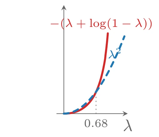
上图由下面的 TikZ 代码编译而来：

  \definecolor{cblue}{RGB}{31,119,180}
  \definecolor{cred}{RGB}{214,39,40}
  \definecolor{cgreen}{RGB}{44,160,44}
  \definecolor{corange}{RGB}{255,127,14}
  \definecolor{cpurple}{RGB}{148,103,189}
  \definecolor{cbrown}{RGB}{140,86,75}
  \definecolor{cpink}{RGB}{227,119,194}
  \definecolor{cgray}{RGB}{127,127,127}
\begin{tikzpicture}[x=1cm,y=1cm,>=stealth,line cap=round,line join=round]
  \draw[->,color=black!60] (-0.15,0) -- (1.35,0) node[below] {$\lambda$};
  \draw[->,color=black!60] (0,0) -- (0,2.3) node[left] {};
  \draw[cred,very thick,domain=0:0.93,samples=100] plot (\x,{-\x-ln(1-\x)});
  \draw[cblue,very thick,dashed,domain=0:1.28] plot (\x,{\x*\x});
  \draw[color=black!55,dotted] (0.68,0) -- (0.68,0.47);
  \node[below,font=\scriptsize,color=black!60] at (0.68,0) {$0.68$};
  \node[font=\scriptsize,color=cred] at (0.79,1.9) {$-(\lambda+\log(1-\lambda))$};
  \node[font=\scriptsize,color=cblue] at (1.08,1.28) {$\lambda^2$};
\end{tikzpicture}

自和谐函数的 Newton 方法分析

现在对应用于严格凸自和谐函数的、带回溯直线搜索的 Newton 方法进行分析。假设已知初始点 $x^{(0)}$，下水平集 $S=\{x\mid f(x)⩽f(x^{(0)})\}$ 是闭集，且 $f$ 下有界（这意味着 $f$ 存在极小点 $x^{\star }$）。该分析与经典分析非常相似，只是以自和谐性代替强凸性和 Hessian 的 Lipschitz 条件，并以 Newton 减量代替梯度范数。可以证明存在只依赖于直线搜索参数 $\alpha$ 和 $\beta$ 的数 $\eta$ 和 $\gamma >0$（$0<\eta ⩽1/4$），使得：

• 若 $\lambda (x^{(k)})>\eta$，则 $f(x^{(k+1)})-f(x^{(k)})⩽-\gamma$；
• 若 $\lambda (x^{(k)})⩽\eta$，则回溯直线搜索选择 $t=1$，且

$$2\lambda (x^{(k+1)})⩽{(2\lambda (x^{(k)}))}^2$$

与经典分析一样，第二条件可以递归应用：对 $l⩾k$，有 $\lambda (x^{(l)})⩽(1/2{)}^{2^{(l-k)}/2}$ 型的界，进而

$$f(x^{(l)})-p^{\star }⩽\lambda (x^{(l)}{)}^2⩽{\left(\frac{1}{2}\right)}^{2(l-k)+1}$$

因此当 $l-k⩾{\log }_2{\log }_2(1/ϵ)$ 时 $f(x^{(l)})-p^{\star }⩽ϵ$。第一条不等式意味着阻尼阶段至多需要 $(f(x^{(0)})-p^{\star })/\gamma$ 步。所以，从 $x^{(0)}$ 出发达到精度 $f(x)-p^{\star }⩽ϵ$ 所需的总迭代次数由下式界定：

$$\frac{f(x^{(0)})-p^{\star }}{\gamma }+{\log }_2{\log }_2(1/ϵ)$$

这正是经典分析中相应界的自和谐版本。

阻尼 Newton 阶段

令 $\tilde{f}(t)=f(x+t\mathrm{\Delta }{x}_{\mathrm{nt}})$，则 ${\tilde{f}}^{\prime }(0)=-\lambda (x{)}^2$，${\tilde{f}}^{″}(0)=\lambda (x{)}^2$。对二阶导数上界积分两次可得（对 $0⩽t<1/\lambda (x)$ 有效）

$$\tilde{f}(t)⩽\tilde{f}(0)-t\lambda (x{)}^2-t\lambda (x)-\log (1-t\lambda (x))$$

利用它可以证明回溯直线搜索得到的步长总满足 $t⩾\beta /(1+\lambda (x))$：点 $\hat{t}=1/(1+\lambda (x))$ 满足直线搜索终止条件（利用对 $x⩾0$ 成立的不等式 $-x+\log (1+x)+\frac{x^2}{2(1+x)}⩽0$）。于是

$$\tilde{f}(t)-\tilde{f}(0)⩽-\alpha \beta \frac{\lambda (x{)}^2}{1+\lambda (x)}$$

即第一条性质成立，且 $\gamma =\alpha \beta {\eta }^2/(1+\eta )$。

二次收敛阶段

可以取 $\eta =(1-2\alpha )/4$（因 $0<\alpha <1/2$，它满足 $0<\eta <1/4$）：若 $\lambda (x^{(k)})⩽(1-2\alpha )/4$，则回溯直线搜索接受单位步长，且第二条性质成立。事实上，上述 $\tilde{f}$ 的上界表明：单位步长 $t=1$ 在 $\lambda (x)<1$ 时产生定义域内的点；而当 $\lambda (x)⩽(1-2\alpha )/2$ 时 $\tilde{f}(1)⩽\tilde{f}(0)-\alpha \lambda (x{)}^2$，满足充分下降条件。至于 $\lambda$ 的递减，有如下事实（见教材习题 9.18）：若 $\lambda (x)<1$ 且 $x^{+}=x-{\mathrm{\nabla }}^{2}f(x{)}^{-1}\mathrm{\nabla }f(x)$，则

$$\lambda (x^{+})⩽\frac{\lambda (x{)}^2}{(1-\lambda (x){)}^2}$$

特别地，当 $\lambda (x)⩽1/4$ 时 $\lambda (x^{+})⩽2\lambda (x{)}^2$，这就证明了 $\lambda (x^{(k)})⩽\eta$ 时第二条性质成立。

最终复杂度界

综合起来，总迭代次数的界为

$$\frac{20-8\alpha }{\alpha \beta (1-2\alpha {)}^2}(f(x^{(0)})-p^{\star })+{\log }_2{\log }_2(1/ϵ)$$

这个表达式只依赖于直线搜索参数 $\alpha$、$\beta$ 和最终精度 $ϵ$；其中与 $ϵ$ 有关的一项可以放心地用常数 6 代替。对典型的 $\alpha$、$\beta$，缩放 $f(x^{(0)})-p^{\star }$ 的常数是几百的量级：例如 $\alpha =0.1$、$\beta =0.8$ 时该常数为 375，取 $ϵ={10}^{-10}$ 得到界

$$375(f(x^{(0)})-p^{\star })+6$$

这个界相当保守，但确实刻画了 Newton 步数的（最坏情形）一般形式。更精细的分析（如 Nesterov 和 Nemirovski 的原始分析）给出类似形式的界，但缩放常数小得多。

讨论与数值例子

一族自和谐函数

把上界与实际迭代次数进行比较是有意义的。考虑问题族 $f(x)=-\sum _{i=1}^m\log (b_i-a_i^{\mathrm{\top }}x)$（随机生成数据，剔除下无界的实例）。对每个实例先计算 $x^{\star }$，再沿随机方向取初始点使 $f(x^{(0)})-p^{\star }$ 为 0 到 35 之间的给定值，然后用参数 $\alpha =0.1$、$\beta =0.8$、容许误差 $ϵ={10}^{-10}$ 的 Newton 方法极小化。

150 个实例的结果显示：实际所需 Newton 步数远小于界 $375(f(x^{(0)})-p^{\star })+6$。结果暗示存在形如相同、但常数小得多（约 1.5）的界。事实上，表达式

$$f(x^{(0)})-p^{\star }+6$$

作为所需 Newton 步数的粗略预测效果并不差（尽管它显然不是唯一因素）。还应指出，所研究的问题族不仅是自和谐的，而且是极小自和谐​（minimally self-concordant）的——即对 $\alpha <1$，$\alpha f$ 不再自和谐——因此该界无法通过缩放 $f$ 来改进。（$f(x)=-20\log x$ 是一个自和谐但非极小自和谐的函数的例子，因为 $(1/20)f$ 也自和谐。）

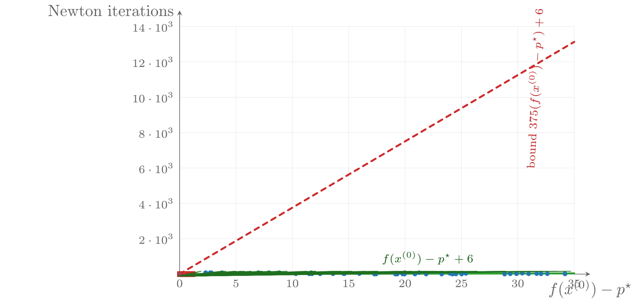
上图由下面的 TikZ 代码编译而来：

  \definecolor{cblue}{RGB}{31,119,180}
  \definecolor{cred}{RGB}{214,39,40}
  \definecolor{cgreen}{RGB}{44,160,44}
  \definecolor{corange}{RGB}{255,127,14}
  \definecolor{cpurple}{RGB}{148,103,189}
  \definecolor{cbrown}{RGB}{140,86,75}
  \definecolor{cpink}{RGB}{227,119,194}
  \definecolor{cgray}{RGB}{127,127,127}
\begin{tikzpicture}[x=1cm,y=1cm,>=stealth,line cap=round,line join=round]
  \draw[color=black!12,very thin] (0.0000,0) -- (0.0000,5.4) (1.2286,0) -- (1.2286,5.4) (2.4571,0) -- (2.4571,5.4) (3.6857,0) -- (3.6857,5.4) (4.9143,0) -- (4.9143,5.4) (6.1429,0) -- (6.1429,5.4) (7.3714,0) -- (7.3714,5.4) (8.6000,0) -- (8.6000,5.4) (0,0.7714) -- (8.6,0.7714) (0,1.5429) -- (8.6,1.5429) (0,2.3143) -- (8.6,2.3143) (0,3.0857) -- (8.6,3.0857) (0,3.8571) -- (8.6,3.8571) (0,4.6286) -- (8.6,4.6286) (0,5.4000) -- (8.6,5.4000) ;
  \draw[->,color=black!60] (0,0) -- (8.95,0) node[below] {$f(x^{(0)})-p^{\star}$};
  \draw[->,color=black!60] (0,0) -- (0,5.75) node[left] {Newton iterations};
  \draw[cred,very thick,dashed] (0,0.0023) -- (8.6000,5.0648);
  \draw[cgreen,very thick] (0,0.0023) -- (8.6000,0.0158);
  \fill[cblue] (4.7044,0.0004) circle (1.4pt);
  \fill[cblue] (2.1678,0.0309) circle (1.4pt);
  \fill[cblue] (3.5937,0.0093) circle (1.4pt);
  \fill[cblue] (6.1471,0.0012) circle (1.4pt);
  \fill[cblue] (4.2844,0.0023) circle (1.4pt);
  \fill[cblue] (7.0840,0.0000) circle (1.4pt);
  \fill[cblue] (4.9066,0.0309) circle (1.4pt);
  \fill[cblue] (7.7836,0.0100) circle (1.4pt);
  \fill[cblue] (4.7417,0.0004) circle (1.4pt);
  \fill[cblue] (7.4681,0.0197) circle (1.4pt);
  \fill[cblue] (7.8778,0.0062) circle (1.4pt);
  \fill[cblue] (0.5719,0.0309) circle (1.4pt);
  \fill[cblue] (3.9173,0.0108) circle (1.4pt);
  \fill[cblue] (8.4017,0.0039) circle (1.4pt);
  \fill[cblue] (3.5754,0.0093) circle (1.4pt);
  \fill[cblue] (2.8234,0.0077) circle (1.4pt);
  \fill[cblue] (5.7121,0.0012) circle (1.4pt);
  \fill[cblue] (0.0591,0.0012) circle (1.4pt);
  \fill[cblue] (2.8308,0.0077) circle (1.4pt);
  \fill[cblue] (0.0241,0.0012) circle (1.4pt);
  \fill[cblue] (7.6071,0.0073) circle (1.4pt);
  \fill[cblue] (5.8901,0.0158) circle (1.4pt);
  \fill[cblue] (5.3736,0.0008) circle (1.4pt);
  \fill[cblue] (0.9279,0.0309) circle (1.4pt);
  \fill[cblue] (5.9459,0.0000) circle (1.4pt);
  \fill[cblue] (3.0619,0.0069) circle (1.4pt);
  \fill[cblue] (2.8675,0.0309) circle (1.4pt);
  \fill[cblue] (4.9083,0.0116) circle (1.4pt);
  \fill[cblue] (0.5662,0.0027) circle (1.4pt);
  \fill[cblue] (0.6661,0.0309) circle (1.4pt);
  \fill[cblue] (2.5339,0.0073) circle (1.4pt);
  \fill[cblue] (4.8981,0.0000) circle (1.4pt);
  \fill[cblue] (5.9426,0.0139) circle (1.4pt);
  \fill[cblue] (8.0155,0.0085) circle (1.4pt);
  \fill[cblue] (5.1292,0.0008) circle (1.4pt);
  \fill[cblue] (1.7141,0.0309) circle (1.4pt);
  \fill[cblue] (5.9506,0.0027) circle (1.4pt);
  \fill[cblue] (0.5651,0.0309) circle (1.4pt);
  \fill[cblue] (4.2469,0.0000) circle (1.4pt);
  \fill[cblue] (6.0213,0.0019) circle (1.4pt);
  \fill[cblue] (7.3427,0.0066) circle (1.4pt);
  \fill[cblue] (7.2065,0.0062) circle (1.4pt);
  \fill[cblue] (6.2388,0.0143) circle (1.4pt);
  \fill[cblue] (1.9455,0.0309) circle (1.4pt);
  \fill[cblue] (2.8860,0.0066) circle (1.4pt);
  \fill[cblue] (8.3969,0.0093) circle (1.4pt);
  \fill[cblue] (5.2183,0.0309) circle (1.4pt);
  \fill[cblue] (4.8605,0.0031) circle (1.4pt);
  \fill[cblue] (0.6934,0.0309) circle (1.4pt);
  \fill[cblue] (3.3424,0.0069) circle (1.4pt);
  \draw[cred] (2.4283-1.5pt,0.0031-1.5pt) rectangle ++(3pt,3pt);
  \draw[cred] (0.1145-1.5pt,0.0015-1.5pt) rectangle ++(3pt,3pt);
  \draw[cred] (0.2111-1.5pt,0.0015-1.5pt) rectangle ++(3pt,3pt);
  \draw[cred] (7.8808-1.5pt,0.0220-1.5pt) rectangle ++(3pt,3pt);
  \draw[cred] (4.4440-1.5pt,0.0077-1.5pt) rectangle ++(3pt,3pt);
  \draw[cred] (7.2865-1.5pt,0.0004-1.5pt) rectangle ++(3pt,3pt);
  \draw[cred] (4.1371-1.5pt,0.0108-1.5pt) rectangle ++(3pt,3pt);
  \draw[cred] (6.7669-1.5pt,0.0004-1.5pt) rectangle ++(3pt,3pt);
  \draw[cred] (6.9121-1.5pt,0.0000-1.5pt) rectangle ++(3pt,3pt);
  \draw[cred] (0.7004-1.5pt,0.0019-1.5pt) rectangle ++(3pt,3pt);
  \draw[cred] (5.6065-1.5pt,0.0077-1.5pt) rectangle ++(3pt,3pt);
  \draw[cred] (7.9570-1.5pt,0.0120-1.5pt) rectangle ++(3pt,3pt);
  \draw[cred] (0.4628-1.5pt,0.0015-1.5pt) rectangle ++(3pt,3pt);
  \draw[cred] (6.6335-1.5pt,0.0008-1.5pt) rectangle ++(3pt,3pt);
  \draw[cred] (3.9690-1.5pt,0.0062-1.5pt) rectangle ++(3pt,3pt);
  \draw[cred] (2.3444-1.5pt,0.0023-1.5pt) rectangle ++(3pt,3pt);
  \draw[cred] (5.9134-1.5pt,0.0012-1.5pt) rectangle ++(3pt,3pt);
  \draw[cred] (4.4577-1.5pt,0.0104-1.5pt) rectangle ++(3pt,3pt);
  \draw[cred] (1.0581-1.5pt,0.0031-1.5pt) rectangle ++(3pt,3pt);
  \draw[cred] (5.0829-1.5pt,0.0093-1.5pt) rectangle ++(3pt,3pt);
  \draw[cred] (2.2576-1.5pt,0.0042-1.5pt) rectangle ++(3pt,3pt);
  \draw[cred] (3.1310-1.5pt,0.0073-1.5pt) rectangle ++(3pt,3pt);
  \draw[cred] (7.3053-1.5pt,0.0015-1.5pt) rectangle ++(3pt,3pt);
  \draw[cred] (4.3920-1.5pt,0.0096-1.5pt) rectangle ++(3pt,3pt);
  \draw[cred] (7.7919-1.5pt,0.0000-1.5pt) rectangle ++(3pt,3pt);
  \draw[cred] (2.7890-1.5pt,0.0050-1.5pt) rectangle ++(3pt,3pt);
  \draw[cred] (6.4773-1.5pt,0.0069-1.5pt) rectangle ++(3pt,3pt);
  \draw[cred] (6.6357-1.5pt,0.0073-1.5pt) rectangle ++(3pt,3pt);
  \draw[cred] (6.5298-1.5pt,0.0039-1.5pt) rectangle ++(3pt,3pt);
  \draw[cred] (2.6058-1.5pt,0.0031-1.5pt) rectangle ++(3pt,3pt);
  \draw[cred] (6.4501-1.5pt,0.0023-1.5pt) rectangle ++(3pt,3pt);
  \draw[cred] (6.2948-1.5pt,0.0008-1.5pt) rectangle ++(3pt,3pt);
  \draw[cred] (5.2292-1.5pt,0.0000-1.5pt) rectangle ++(3pt,3pt);
  \draw[cred] (4.9604-1.5pt,0.0089-1.5pt) rectangle ++(3pt,3pt);
  \draw[cred] (7.7055-1.5pt,0.0004-1.5pt) rectangle ++(3pt,3pt);
  \draw[cred] (6.6919-1.5pt,0.0012-1.5pt) rectangle ++(3pt,3pt);
  \draw[cred] (0.5966-1.5pt,0.0019-1.5pt) rectangle ++(3pt,3pt);
  \draw[cred] (5.4008-1.5pt,0.0123-1.5pt) rectangle ++(3pt,3pt);
  \draw[cred] (0.4617-1.5pt,0.0023-1.5pt) rectangle ++(3pt,3pt);
  \draw[cred] (6.6260-1.5pt,0.0000-1.5pt) rectangle ++(3pt,3pt);
  \draw[cred] (5.6788-1.5pt,0.0042-1.5pt) rectangle ++(3pt,3pt);
  \draw[cred] (8.2414-1.5pt,0.0023-1.5pt) rectangle ++(3pt,3pt);
  \draw[cred] (6.3240-1.5pt,0.0015-1.5pt) rectangle ++(3pt,3pt);
  \draw[cred] (3.4010-1.5pt,0.0077-1.5pt) rectangle ++(3pt,3pt);
  \draw[cred] (4.1282-1.5pt,0.0069-1.5pt) rectangle ++(3pt,3pt);
  \draw[cred] (3.2177-1.5pt,0.0031-1.5pt) rectangle ++(3pt,3pt);
  \draw[cred] (4.9990-1.5pt,0.0089-1.5pt) rectangle ++(3pt,3pt);
  \draw[cred] (2.7311-1.5pt,0.0066-1.5pt) rectangle ++(3pt,3pt);
  \draw[cred] (2.9397-1.5pt,0.0054-1.5pt) rectangle ++(3pt,3pt);
  \draw[cred] (4.2887-1.5pt,0.0089-1.5pt) rectangle ++(3pt,3pt);
  \draw[fill] [cgreen!70!black] (3.3668,0.0015+1.8pt) -- (3.3668-1.7pt,0.0015-1.2pt) -- (3.3668+1.7pt,0.0015-1.2pt) -- cycle;
  \draw[fill] [cgreen!70!black] (5.7448,0.0019+1.8pt) -- (5.7448-1.7pt,0.0019-1.2pt) -- (5.7448+1.7pt,0.0019-1.2pt) -- cycle;
  \draw[fill] [cgreen!70!black] (4.2805,0.0015+1.8pt) -- (4.2805-1.7pt,0.0015-1.2pt) -- (4.2805+1.7pt,0.0015-1.2pt) -- cycle;
  \draw[fill] [cgreen!70!black] (2.2077,0.0023+1.8pt) -- (2.2077-1.7pt,0.0023-1.2pt) -- (2.2077+1.7pt,0.0023-1.2pt) -- cycle;
  \draw[fill] [cgreen!70!black] (5.3533,0.0054+1.8pt) -- (5.3533-1.7pt,0.0054-1.2pt) -- (5.3533+1.7pt,0.0054-1.2pt) -- cycle;
  \draw[fill] [cgreen!70!black] (5.4352,0.0069+1.8pt) -- (5.4352-1.7pt,0.0069-1.2pt) -- (5.4352+1.7pt,0.0069-1.2pt) -- cycle;
  \draw[fill] [cgreen!70!black] (5.6007,0.0042+1.8pt) -- (5.6007-1.7pt,0.0042-1.2pt) -- (5.6007+1.7pt,0.0042-1.2pt) -- cycle;
  \draw[fill] [cgreen!70!black] (8.0243,0.0027+1.8pt) -- (8.0243-1.7pt,0.0027-1.2pt) -- (8.0243+1.7pt,0.0027-1.2pt) -- cycle;
  \draw[fill] [cgreen!70!black] (3.7085,0.0023+1.8pt) -- (3.7085-1.7pt,0.0023-1.2pt) -- (3.7085+1.7pt,0.0023-1.2pt) -- cycle;
  \draw[fill] [cgreen!70!black] (3.4342,0.0023+1.8pt) -- (3.4342-1.7pt,0.0023-1.2pt) -- (3.4342+1.7pt,0.0023-1.2pt) -- cycle;
  \draw[fill] [cgreen!70!black] (0.4685,0.0015+1.8pt) -- (0.4685-1.7pt,0.0015-1.2pt) -- (0.4685+1.7pt,0.0015-1.2pt) -- cycle;
  \draw[fill] [cgreen!70!black] (4.7816,0.0023+1.8pt) -- (4.7816-1.7pt,0.0023-1.2pt) -- (4.7816+1.7pt,0.0023-1.2pt) -- cycle;
  \draw[fill] [cgreen!70!black] (6.4864,0.0054+1.8pt) -- (6.4864-1.7pt,0.0054-1.2pt) -- (6.4864+1.7pt,0.0054-1.2pt) -- cycle;
  \draw[fill] [cgreen!70!black] (7.8721,0.0062+1.8pt) -- (7.8721-1.7pt,0.0062-1.2pt) -- (7.8721+1.7pt,0.0062-1.2pt) -- cycle;
  \draw[fill] [cgreen!70!black] (4.3222,0.0066+1.8pt) -- (4.3222-1.7pt,0.0066-1.2pt) -- (4.3222+1.7pt,0.0066-1.2pt) -- cycle;
  \draw[fill] [cgreen!70!black] (8.2162,0.0131+1.8pt) -- (8.2162-1.7pt,0.0131-1.2pt) -- (8.2162+1.7pt,0.0131-1.2pt) -- cycle;
  \draw[fill] [cgreen!70!black] (6.1820,0.0023+1.8pt) -- (6.1820-1.7pt,0.0023-1.2pt) -- (6.1820+1.7pt,0.0023-1.2pt) -- cycle;
  \draw[fill] [cgreen!70!black] (3.7577,0.0023+1.8pt) -- (3.7577-1.7pt,0.0023-1.2pt) -- (3.7577+1.7pt,0.0023-1.2pt) -- cycle;
  \draw[fill] [cgreen!70!black] (3.5177,0.0027+1.8pt) -- (3.5177-1.7pt,0.0027-1.2pt) -- (3.5177+1.7pt,0.0027-1.2pt) -- cycle;
  \draw[fill] [cgreen!70!black] (1.5618,0.0019+1.8pt) -- (1.5618-1.7pt,0.0019-1.2pt) -- (1.5618+1.7pt,0.0019-1.2pt) -- cycle;
  \draw[fill] [cgreen!70!black] (1.7782,0.0019+1.8pt) -- (1.7782-1.7pt,0.0019-1.2pt) -- (1.7782+1.7pt,0.0019-1.2pt) -- cycle;
  \draw[fill] [cgreen!70!black] (2.9688,0.0062+1.8pt) -- (2.9688-1.7pt,0.0062-1.2pt) -- (2.9688+1.7pt,0.0062-1.2pt) -- cycle;
  \draw[fill] [cgreen!70!black] (7.5594,0.0031+1.8pt) -- (7.5594-1.7pt,0.0031-1.2pt) -- (7.5594+1.7pt,0.0031-1.2pt) -- cycle;
  \draw[fill] [cgreen!70!black] (5.3840,0.0069+1.8pt) -- (5.3840-1.7pt,0.0069-1.2pt) -- (5.3840+1.7pt,0.0069-1.2pt) -- cycle;
  \draw[fill] [cgreen!70!black] (1.9852,0.0015+1.8pt) -- (1.9852-1.7pt,0.0015-1.2pt) -- (1.9852+1.7pt,0.0015-1.2pt) -- cycle;
  \draw[fill] [cgreen!70!black] (6.4825,0.0077+1.8pt) -- (6.4825-1.7pt,0.0077-1.2pt) -- (6.4825+1.7pt,0.0077-1.2pt) -- cycle;
  \draw[fill] [cgreen!70!black] (5.5232,0.0054+1.8pt) -- (5.5232-1.7pt,0.0054-1.2pt) -- (5.5232+1.7pt,0.0054-1.2pt) -- cycle;
  \draw[fill] [cgreen!70!black] (1.2241,0.0015+1.8pt) -- (1.2241-1.7pt,0.0015-1.2pt) -- (1.2241+1.7pt,0.0015-1.2pt) -- cycle;
  \draw[fill] [cgreen!70!black] (2.7770,0.0023+1.8pt) -- (2.7770-1.7pt,0.0023-1.2pt) -- (2.7770+1.7pt,0.0023-1.2pt) -- cycle;
  \draw[fill] [cgreen!70!black] (1.4128,0.0015+1.8pt) -- (1.4128-1.7pt,0.0015-1.2pt) -- (1.4128+1.7pt,0.0015-1.2pt) -- cycle;
  \draw[fill] [cgreen!70!black] (8.5283,0.0008+1.8pt) -- (8.5283-1.7pt,0.0008-1.2pt) -- (8.5283+1.7pt,0.0008-1.2pt) -- cycle;
  \draw[fill] [cgreen!70!black] (1.1993,0.0015+1.8pt) -- (1.1993-1.7pt,0.0015-1.2pt) -- (1.1993+1.7pt,0.0015-1.2pt) -- cycle;
  \draw[fill] [cgreen!70!black] (2.1589,0.0023+1.8pt) -- (2.1589-1.7pt,0.0023-1.2pt) -- (2.1589+1.7pt,0.0023-1.2pt) -- cycle;
  \draw[fill] [cgreen!70!black] (7.6810,0.0019+1.8pt) -- (7.6810-1.7pt,0.0019-1.2pt) -- (7.6810+1.7pt,0.0019-1.2pt) -- cycle;
  \draw[fill] [cgreen!70!black] (4.9430,0.0019+1.8pt) -- (4.9430-1.7pt,0.0019-1.2pt) -- (4.9430+1.7pt,0.0019-1.2pt) -- cycle;
  \draw[fill] [cgreen!70!black] (5.0673,0.0089+1.8pt) -- (5.0673-1.7pt,0.0089-1.2pt) -- (5.0673+1.7pt,0.0089-1.2pt) -- cycle;
  \draw[fill] [cgreen!70!black] (3.4997,0.0039+1.8pt) -- (3.4997-1.7pt,0.0039-1.2pt) -- (3.4997+1.7pt,0.0039-1.2pt) -- cycle;
  \draw[fill] [cgreen!70!black] (7.9318,0.0069+1.8pt) -- (7.9318-1.7pt,0.0069-1.2pt) -- (7.9318+1.7pt,0.0069-1.2pt) -- cycle;
  \draw[fill] [cgreen!70!black] (4.9003,0.0031+1.8pt) -- (4.9003-1.7pt,0.0031-1.2pt) -- (4.9003+1.7pt,0.0031-1.2pt) -- cycle;
  \draw[fill] [cgreen!70!black] (2.3444,0.0019+1.8pt) -- (2.3444-1.7pt,0.0019-1.2pt) -- (2.3444+1.7pt,0.0019-1.2pt) -- cycle;
  \draw[fill] [cgreen!70!black] (6.0222,0.0096+1.8pt) -- (6.0222-1.7pt,0.0096-1.2pt) -- (6.0222+1.7pt,0.0096-1.2pt) -- cycle;
  \draw[fill] [cgreen!70!black] (1.8045,0.0015+1.8pt) -- (1.8045-1.7pt,0.0015-1.2pt) -- (1.8045+1.7pt,0.0015-1.2pt) -- cycle;
  \draw[fill] [cgreen!70!black] (0.9110,0.0015+1.8pt) -- (0.9110-1.7pt,0.0015-1.2pt) -- (0.9110+1.7pt,0.0015-1.2pt) -- cycle;
  \draw[fill] [cgreen!70!black] (4.9424,0.0058+1.8pt) -- (4.9424-1.7pt,0.0058-1.2pt) -- (4.9424+1.7pt,0.0058-1.2pt) -- cycle;
  \draw[fill] [cgreen!70!black] (1.0088,0.0015+1.8pt) -- (1.0088-1.7pt,0.0015-1.2pt) -- (1.0088+1.7pt,0.0015-1.2pt) -- cycle;
  \draw[fill] [cgreen!70!black] (7.0499,0.0116+1.8pt) -- (7.0499-1.7pt,0.0116-1.2pt) -- (7.0499+1.7pt,0.0116-1.2pt) -- cycle;
  \draw[fill] [cgreen!70!black] (7.1144,0.0058+1.8pt) -- (7.1144-1.7pt,0.0058-1.2pt) -- (7.1144+1.7pt,0.0058-1.2pt) -- cycle;
  \draw[fill] [cgreen!70!black] (1.3419,0.0015+1.8pt) -- (1.3419-1.7pt,0.0015-1.2pt) -- (1.3419+1.7pt,0.0015-1.2pt) -- cycle;
  \draw[fill] [cgreen!70!black] (4.0596,0.0019+1.8pt) -- (4.0596-1.7pt,0.0019-1.2pt) -- (4.0596+1.7pt,0.0019-1.2pt) -- cycle;
  \draw[fill] [cgreen!70!black] (8.4935,0.0108+1.8pt) -- (8.4935-1.7pt,0.0108-1.2pt) -- (8.4935+1.7pt,0.0108-1.2pt) -- cycle;
  \node[below,font=\scriptsize,color=black!60] at (0.0000,0) {0};
  \node[below,font=\scriptsize,color=black!60] at (1.2286,0) {5};
  \node[below,font=\scriptsize,color=black!60] at (2.4571,0) {10};
  \node[below,font=\scriptsize,color=black!60] at (3.6857,0) {15};
  \node[below,font=\scriptsize,color=black!60] at (4.9143,0) {20};
  \node[below,font=\scriptsize,color=black!60] at (6.1429,0) {25};
  \node[below,font=\scriptsize,color=black!60] at (7.3714,0) {30};
  \node[below,font=\scriptsize,color=black!60] at (8.6000,0) {35};
  \node[left,font=\scriptsize,color=black!60] at (0,0.7714) {$2\cdot 10^{3}$};
  \node[left,font=\scriptsize,color=black!60] at (0,1.5429) {$4\cdot 10^{3}$};
  \node[left,font=\scriptsize,color=black!60] at (0,2.3143) {$6\cdot 10^{3}$};
  \node[left,font=\scriptsize,color=black!60] at (0,3.0857) {$8\cdot 10^{3}$};
  \node[left,font=\scriptsize,color=black!60] at (0,3.8571) {$10\cdot 10^{3}$};
  \node[left,font=\scriptsize,color=black!60] at (0,4.6286) {$12\cdot 10^{3}$};
  \node[left,font=\scriptsize,color=black!60] at (0,5.4000) {$14\cdot 10^{3}$};
  \node[font=\scriptsize,color=cred,rotate=87] at (7.7400,4.0500) {bound $375(f(x^{(0)})-p^{\star})+6$};
  \node[font=\scriptsize,color=cgreen!60!black] at (5.4057,0.3471) {$f(x^{(0)})-p^{\star}+6$};
\end{tikzpicture}

自和谐性的实际意义

我们已经看到，Newton 方法对强凸目标函数一般表现得非常好；经典分析可以给出复杂度界，但该界依赖几个几乎总是未知的常数。

对自和谐函数可以说得更多：我们有一个完全显式的、不依赖任何未知常数的复杂度界。实证研究表明该界可以大幅收紧，但其一般形式——一个较小的常数加上 $f(x^{(0)})-p^{\star }$ 的某个倍数——至少粗略地预测了极小化一个（近似）极小自和谐函数所需的 Newton 步数。

自和谐函数在实践中是否比非自和谐函数更容易用 Newton 方法极小化，目前还不清楚（甚至不清楚如何把这句话表述得严谨）。目前可以说的是：自和谐函数是这样一类函数，对它们我们关于 Newton 方法复杂度所能说的，比非自和谐函数的情形多得多。